Generative Models - Part I VAE

(Migrated from old blog)

In Generative Models, we generate data based on the distribution of the sample data. basically, we want to learn $ p_{model}(x) $ which is similar to $ p_{data} (x) $ where $ p_{data}(x) $ is the distribution of training data and $ p_{model}(x) $ is the distribution of the model. It addresses the density estimation problem.

Why Generative Models?

All types of generative models aim at learning the true data distribution of the training set so as to generate new data points with some variations. Which is a very powerful thing because of this we can approximate true probability of the distribution hence, we can generate realistic data.

Generating Real life sceneries from doodles

Colorization of Objects using GAN

These are one of the practical applications of Generative Models, these models are also widely used for medical imaging purposes since there are few datasets present for some rare diseases also, Generative Models of Time Series can also be used for simulation and planning and many many more applications.

Generative Models are of Two Types :

1.) Explicit Density Estimators: Where we explicitly define and solve for $ p_{model}(x) $ like PixelRNN/CNN, Variational Autoencoders 2.) Implicit Density: We learn a model that can learn $ p_{model}(x) $ without explicitly mentioning its distribution like GAN

PixelRNN and PixelCNN

We have a full belief network, we use a chain rule to decompose the likelihood of an image x into a product of 1-d distribution.

\[p(x) = \prod^n_{i=1} p\left(x_i \vert x_1, \dots, x_{i-1} \right)\]

where $ p(x) $ is probability where the likelihood of an i’th pixel which depends on the probability of the pixel values of the previous pixels and then we maximize the likelihood of the training data, under this defined density.

We need to define the order of all the previous pixels. In this, we start from the top left corner and then keep on generating the neighboring pixels with an RNN (LSTM) and it depends on the previous pixel modeled. the drawback is that it is slow.

In PixelCNN we use CNN instead of RNN, to generate. Depending on the previous pixel we can model the next region using CNN over a context region.

So in Layman’s term, We predict the next value then we generate a loss function ( here the loss function checks the ground truth image not labels thus it is a form of unsupervised learning) and minimize it until we approximate the true distribution.

• Pros:
  • Can explicitly compute likelihood $ p(x) $ and minimise it.
  • Since we have an expressive likelihood of training data we have good evaluation matrices
  • Good Samples
• Cons:
  • Since it is a sequential Generation, it is slow
  • Images are not sharp much there is a lot of room for improvements

Variational Autoencoders (VAE)

AutoEncoders

Before starting with VAE, let’s learn a little about AutoEncoders. Autoencoders are an unsupervised way of learning lower-dimensional feature representation from unlabeled training data.

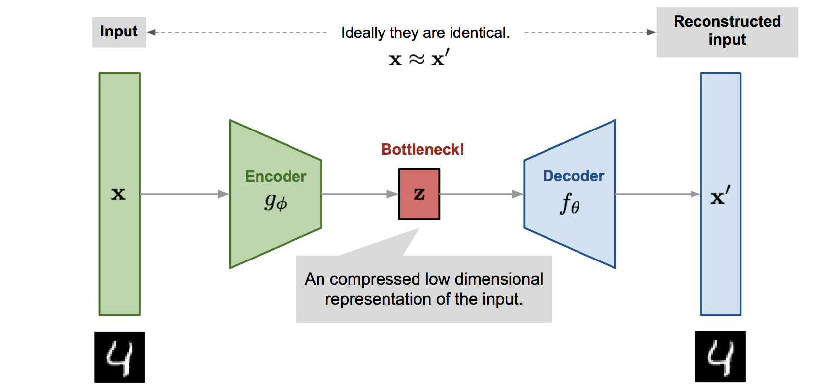Source : https://lilianweng.github.io/lil-log/2018/08/12/from-autoencoder-to-beta-vae.html

The image itself represents a lot we have an input we encode it into a lower-dimensional input and the decoder then regenerates the image with those latent vectors.

But why is it generated in a lower dimension? It is because we want the encoder-decoder network to learn only the most important lower-dimensional details/features, it helps to leave out the noise and the model only remembers important lower-dimensional details. we have a L2 loss function while generating i.e $ \vert \vert x- x\vert \vert ^2 $ still since we don’t use labels it is also a form on unsupervised learning.

Encoder and Decoder are just similar CNN’s in opposite ways like pooling (max) in Encoders and Uppooling in Decoder.

After Training we through away the Decoder and use the encoder to initialize a supervised model. We use this encoded latent vector and predict the labels and then use these predicted labels with the true labels and generate a loss function again fine-tuning the encoder jointly with the classifier.

Now let’s talk about VAE

These are like the probabilistic spin on the Variational Encoders i.e they let us sample from the model to generate data.

We sample from a true pior (example, Gaussian) $ p_{\theta \ast}(z) $ like $ p_{\theta \ast} \left( x \vert z^{\left(i \right)} \right) $ and sample our data $ x $ from here. We want to estimate these parameters $ \theta^\ast $

To represent this model we first need to choose a prior $ p(z) $ like a gaussian distribution. And for conditional distribution $ P(x \vert z) $ i.e generative image, we will use a neural network. It is a decoder network. i.e It will learn from these latent vectors and generate images with those.

We learn model parameters and maximize the likelihood of training data. $ p_{\theta} ( x ) = \int p_{\theta} (z) p_{\theta} (x \vert z ) dz $ But we cannot compute $ p ( x \vert z ) $ for every $ z$ Thus the integral is interactible.

So the solution is to define another encoder network in addition to decoder network $ p_{\theta} ( x \vert z ) $ so the encoder network $ q_{\phi} (z \vert x) $ will now approximate $ p_{\theta} ( z \vert x ) $ , this allows us to derive a lower bound on the likelihood that is now tractable and can be optimized.

Since we are modeling probabilistic data encoder and decoder are probabilistic models

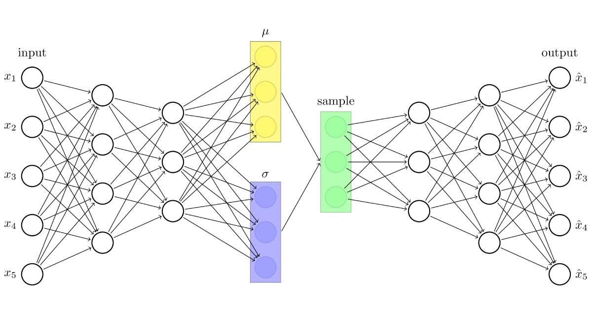
Encoder and Decoder in VAE from “Kingma and Welling “Autoencoding Variational Bayes” ICLR 2014

Now we will sample from these distributions to get the values. i.e sample and generate data.

The idea of VAE is to infer $ p_{\theta} (z) $ using $ p_\theta (z\vert x) $ which we don’t know. We infer $ p_\theta (z\vert x) $ using a method called variational inference which is basically an optimization problem in Bayesian statistics. We first model $ p_\theta (z\vert x) $ using simpler distribution $ q_\phi (z\vert x) $ which is easy to find and we try to minimize the difference between $ p_\theta (z\vert x) $ and $ q_\phi (z\vert x) $ using KL-divergence metric approach so that our hypothesis is close to the true distribution.

By Variational Interference we can find that

\[\log p_{\theta} (x^i) = \mathbf{E}_{z}\left[\log p_{\theta}\left(x^{(i)} \vert z\right)\right]-\mathbf{E}{z}\left[\log \frac{q_{\phi}\left(z \vert x^{(i)}\right)}{p_{\theta}(z)}\right]+\mathbf{E}{z}\left[\log \frac{q_{\phi}\left(z \vert x^{(i)}\right)}{p_{\theta}\left(z \vert x^{(i)}\right)}\right]\]

And we know KL divergence for variational Inference can be written as : $ \mathbf{KL}(q\vert \vert p) = \mathbf{E_q} \left[ \log \frac{ q(z) }{p(z\vert x)} \right] $

Thus the last one’s became :

\[\log p_{\theta} (x^i) = \mathbf{E}_{z}\left[\log p{\theta}\left(x^{(i)} \vert z\right)\right]-D_{K L}\left(q_{\phi}\left(z \vert x^{(i)}\right) \vert \vert p_{\theta}(z)\right)+D_{K L}\left(q_{\phi}\left(z \vert x^{(i)}\right) \vert \vert p_{\theta}\left(z \vert x^{(i)}\right)\right)\]

• $ \mathbf{E}{z}\left\lceil\log p{\theta}\left(x^{(i)} \vert z\right)\right] $ is the decoder network and can be estimated through sampling.
• $ D_{K L}\left(q_{\phi}\left(z \vert x^{(i)}\right) \vert \vert p_{\theta}(z)\right) $ is the KL divergence for the guassian prior $ p_\theta (z) $ and encoder and since both are gaussian the KL divergence will have a nice closed form.
• $ D_{K L}\left(q_{\phi}\left(z \vert x^{(i)}\right) \vert \vert p_{\theta}\left(z \vert x^{(i)}\right)\right) $ We can’t compute this term but we know that Since it is KL divergence it will always be greater than or equal to 0 $ >=0 $

First Two terms are tracktable lower bound or evidence lower bound (ELBO) as reffered in statistics.

Lets call first two terms as

\(\log p_{\theta}\left(x^{(i)}\right) \geq \mathcal{L}\left(x^{(i)}, \theta, \phi\right)\) and in training we maximise this lower bound \(\theta^{}, \phi^{}=\arg \max {\theta, \phi} \sum{i=1}^{N} \mathcal{L}\left(x^{(i)}, \theta, \phi\right)\)

Also, $ \mathbf{E}{z}\left\lceil\log p{\theta}\left(x^{(i)} \vert z\right)\right] $ Can be called as this term reconstructs the input data and $ D_{K L}\left(q_{\phi}\left(z \vert x^{(i)}\right) \vert \vert p_{\theta}(z)\right) $ this term makes approximate posterior information close to prior. Now we can minimise the lower bound and backpropagate and train this model.

Source : https://lilianweng.github.io/lil-log/2018/08/12/from-autoencoder-to-beta-vae.html

Generating Data

We can now use just the Decoder network and sample z from prior.

Writing A Variational Encoder in PyTorch First Lets Import all the libraries needed

import torch
import torch.nn as nn
import torch.nn.functional as F
import torch.optim as optim
from torch.utils.data import DataLoader
from torchvision import datasets, transforms
import matplotlib.pyplot as plt

device = torch.device('cuda' if torch.cuda.is_available() else 'cpu')

Loading the Data, Lets use our favourite dataset MNIST

transformer = transforms.Compose([transforms.ToTensor()])

train_data = datasets.MNIST(root='.data/', train=True, download=True, transform=transformer)
test_data = datasets.MNIST(root='.data/',train=False, download=True, transform=transformer)

Initializing Data Set Iterators for easy and batched access

BATCH_SIZE = 64

train_iterator = DataLoader(train_data, batch_size=BATCH_SIZE, shuffle=True)
test_iterator = DataLoader(test_data, batch_size=BATCH_SIZE)

Now Lets Define the HyperParameters of our VAE Since, VAE is nothing but a combination of Autoencoders, lets define how our architecture will look like

• size of each input
• hidden dimension
• latent vector dimension
• learning rate

INPUT_DIM = 28 * 28
HIDDEN_DIM = 256
LATENT_DIM = 20
lr = 1e-3

In VAE we have one Encoder $ q_\phi (z \vert x) $ , Lets first define that

class Encoder(nn.Module):
    '''
        This is the Encoder of VAE
    '''
    def __init__(self, input_dim, hidden_dim, latent_dim):
        super(Encoder, self).__init__()

        self.linear = nn.Linear(input_dim, hidden_dim)
        self.mu = nn.Linear(hidden_dim, latent_dim)
        self.var = nn.Linear(hidden_dim, latent_dim)

    def forward(self, x):

        hidden = F.relu(self.linear(x))
        mu_z = self.mu(hidden)
        var_z = self.var(hidden)

        return mu_z, var_z

Now, Lets Code Decoder $ p_\theta (x \vert z) $ which will take latent as input and give generated image as output

class Decoder(nn.Module):
    '''
        This is the Decoder part of VAE
    '''
    def __init__(self, latent_dim, hidden_dim, output_dim):
        super(Decoder, self).__init__()
        self.linear = nn.Linear(latent_dim, hidden_dim)
        self.out = nn.Linear(hidden_dim, output_dim)

    def forward(self, x):
        hidden = F.relu(self.linear(x))
        output = torch.sigmoid(self.out(hidden))

        return output

Now we have both our encoder and decoder, Lets write the final architecture of our VAE

class VAE(nn.Module):
    def __init__(self, enc, dec):
        super(VAE, self).__init__()
        self.encoder = enc
        self.decoder = dec

    def sampling(self, mu, var):
        std = torch.exp(var / 2)
        eps = torch.randn_like(std)
        return eps.mul(std).add_(mu)

    def forward(self, x):


        mu_z, var_z = self.encoder(x)

        x_sample = self.sampling(mu_z, var_z)

        prediction = self.decoder(x_sample)

        return prediction, mu_z, var_z

Lets, Initialize the Model

encoder = Encoder(INPUT_DIM, HIDDEN_DIM, LATENT_DIM)
decoder = Decoder(LATENT_DIM, HIDDEN_DIM, INPUT_DIM)

model = VAE(encoder, decoder).to(device)

optimizer = optim.Adam(model.parameters(), lr=lr)

So we know that the LOSS of VAE is the Reconstruction loss and KL Divergence So final loss function will give be = RL + KL

def reconstruction_loss(sampled_input, original_input):
    return F.binary_cross_entropy(sampled_input, original_input, size_average=False)

def kl_divergence(mu_z, var_z):
    return 0.5 * torch.sum(torch.exp(var_z) + mu_z**2 - 1.0 - var_z)

Lets now Train the Model

def train(model, iterator, optimizer):
    model.train()

    train_loss = 0

    for i, (x, _) in enumerate(iterator):
        # Update the size of array
        x = x.view(-1, INPUT_DIM).to(device)

        # Forward Prop
        x_sample, mu_z, var_z = model(x)

        # Calculating Loss
        loss = reconstruction_loss(x_sample, x) + kl_divergence(mu_z, var_z)

        # Backpropagate
        loss.backward()

        # Update Train_loss
        train_loss += loss.item()

        optimizer.step()

    return train_loss

def test(model, iterator, optimizer):
    model.eval()

    test_loss = 0

    with torch.no_grad():
        for i, (x, _) in enumerate(iterator):
            x = x.view(-1, INPUT_DIM).to(device)

            x_sample, mu_z, var_z = model(x)

            loss = reconstruction_loss(x_sample, x) + kl_divergence(mu_z, var_z)

            test_loss += loss.item()

    return test_loss

Finally Training the Model with iterators and dataset

N_EPOCHS = 20
for epoch in range(N_EPOCHS):

        train_loss = train(model, train_iterator, optimizer)
        test_loss = test(model, test_iterator, optimizer)

        train_loss /= len(train_data)
        test_loss /= len(test_data)

        print('Epoch :{}, Train_loss : {} Test_loss: {}'.format(epoch + 1, train_loss, test_loss))

We will get output by

z = torch.randn(1, LATENT_DIM).to(device)

# run only the decoder
reconstructed_img = model.decoder(z)
img = reconstructed_img.view(28, 28).data

print(z.shape)
print(img.shape)
plt.imshow(img.cpu(), cmap='gray')

See this Code in action at Github here : https://github.com/shivammehta25/NLPResearch/blob/master/Tutorials/Generative%20Models/VAE.ipynb

More part with GAN will follow soon