Logistic regression - the math behind it

(Migrated from old blog)

Logistic Regression, unlike Linear Regression, does not output a numerical value but instead outputs a classified output, for example, it can tell whether an email is Spam or Not Spam.

So the input of logistic regression is a x dimentional vector $x ; x \in \mathbb{R}^{n_x} $ and predcits the output $\hat{y} = P(y=1 \vert x) $ i.e probability of y = 1 when given input features x are provided.

Parameters of Logistic Regression: $w ; w \in \mathbb{R}^{n_x} $ and $b \in \mathbb{R} $

In case of linear regression, the output is calculated as \(\hat{y} = w^Tx + b\) while in case of logistic we wrap it around with a sigmoid function,

\[\sigma(y) = \frac{1}{1+e^{-x}}\]

if z is large it will be close to 1 and if it is small or negative it will be close to 0 which is an ideal case for probabilities in case of logistic regression.

A sigmoid function looks like this

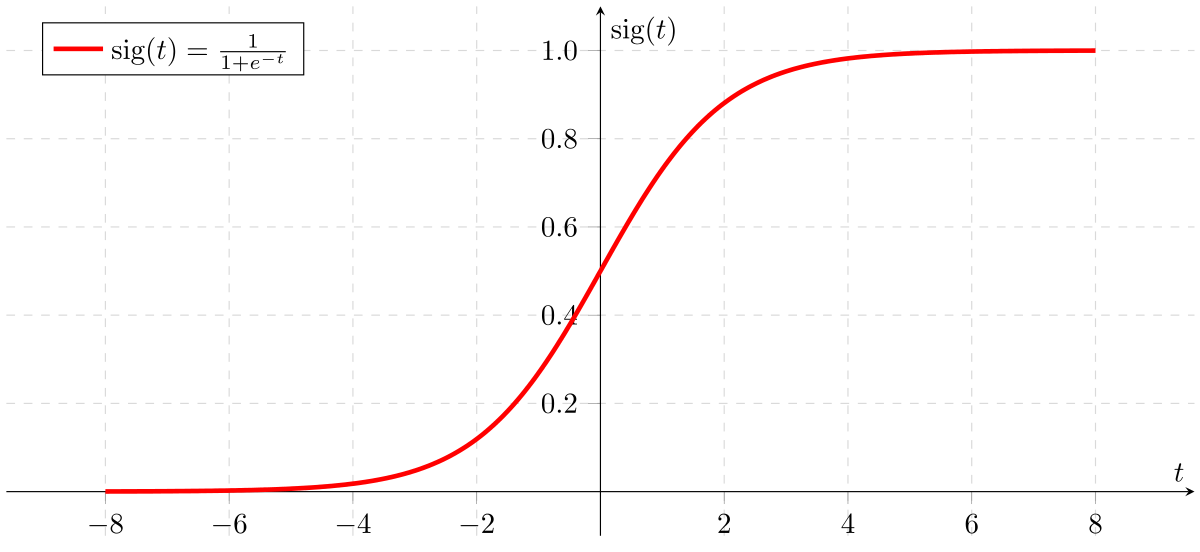Sigmoid function

Now, To train a logistic regression model we need to define a Cost Function

Cost Function

One of the cost function of linear regression \(L(\hat{y},y) = \frac{1}{2}(\hat{y} - y)^2\) but it won’t work in case of linear regression because the optimization problem becomes non convex, maybe we never find the global minimum and be stuck in only local minimum.

So we use loss function : \(L(\hat{y}, y) = -\left(y \log\hat{y} + (1-y)\log(1 -\hat{y})\right)\) Why this loss function ? : \(\text{if } y = 1 ; L(\hat{y}, y) = -\log{\hat{y}}\) i.e we want it to be as max as possible and \(\text{if } y=0; L(\hat{y}, y) = -\log(1-\hat{y})\) i.e we try to make loss function small. This is called as Rafidah’s effect.

So, the final Cost function is, \(J(w,b) = \frac{1}{m} \sum_{i=1}^{m} L\left({\hat{y}}^{(i)}, y^{(i)}\right)\)

So, the final cost function is \(J(w,b) =\frac{1}{m} \sum_{i=1}^{m} -\left( y^{(i)} \log(\hat{y}^{(i)}) + (1-y^{(i)})\log(1-\hat{y}^{(i)}) \right)\)

Gradient Descent

It is one of the methods to optimize an algorithm, where we take step derivate of the cost function and add it with a learning rate to the previous weights. What it means is that, \(w = w - \alpha \frac{d(J)}{dw} = w - \alpha dw\) where dw depicts the slope of the function.

So J(w,b) in w will be \(w = w - \alpha \frac{\partial J(w,b)}{\partial w}\) and for b will be \(b = b- \alpha \frac{\partial J(w,b)}{\partial b}\)

Doing this for logistic regression:

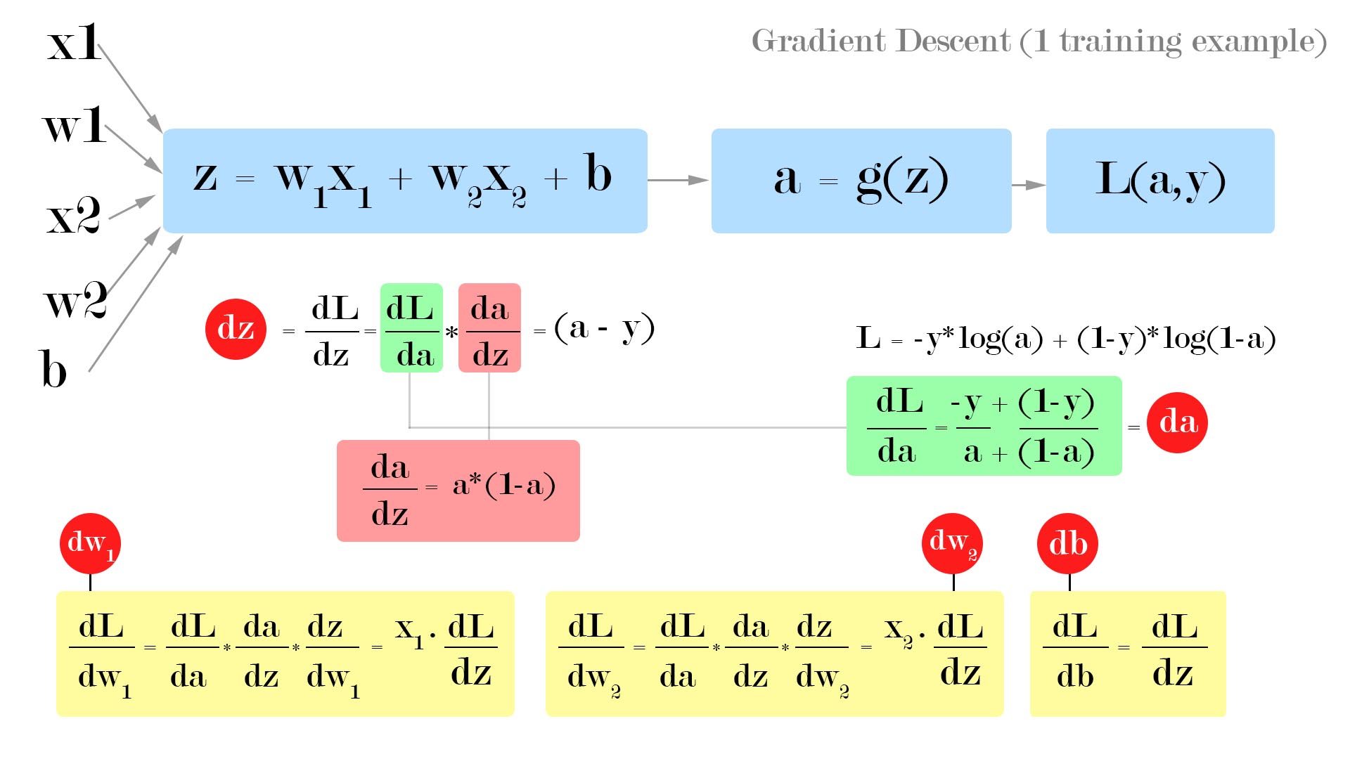
We have equations as, For one example, \(z = w^T \cdot x+ b \tag{1}\) \(\hat{y} = a = \sigma(z) \tag{2}\) and \(L(a,y) = -\left( y\log{a} + (1-y)\log(1-a)\right) \tag{3}\)

Let’s assume we have only two features \(x_1\) and \(x_2\) so, the equation becomes: \(z = w_1 x_1 + w_2 x_2 + b \tag{4}\) We start the backward propagation, to compute effect of \(x_1,w_1,x_2,w_2,b\) on the final loss function $L(a,y)$ we start by computing the derivation of (3) wrt a i.e the output of 2nd equation that is one layer behind.

So the Architecture looks something like this …

Gradient descent

We get,

\(\frac{\partial L(a,y)}{\partial a} = \partial a = - \frac{y}{a} + \frac{1-y}{1-a}\)
now computing the more behind equation i.e (2)
\(\partial z = \frac{\partial L(a,y)}{\partial z} = a- y = \frac{\partial L}{\partial a} \times \frac{\partial a}{\partial z}\)
where \(\frac{\partial a}{\partial z} = a(1-a)\)
which is the derivative of the sigmoid function.

Therefore \(\frac{\partial L}{\partial w_1} = \partial w_1 = x_1 \partial z\) Similarly, \(\frac{\partial L}{\partial w_2} = \partial w_1 = x_2 \partial z\) and \(\frac{\partial L}{\partial b} = \partial b = \partial z\)

So the Algorithm Goes like this for each epoch of back propagation:

j = 0 , dw1 = 0 , dw2 = 0 , db = 0
for i=1 to m:
    z[i] = W.T*x + b
    a[i] = sigmoid(z[i])
    j += - ( y[i] * log(a[i]) + (1 - y[i]) log (1 - a[i]))
    dz[i] = a[i] - y[i]
    dw1 += x1[i] - dz[i]
    dw2 += x2[i] - dz[i]
    db  += dz[i]

j /= m
dw1 /= m
dw2 /= m
db /= m

w1 = w1 - alpha * dw1
w2 = w2 - alpha * dw2
b = b - alpha * db