
(Migrated from old blog)
As the name suggests topic modeling refers to the determination of the topic of the text. Imagine creating a news platform where the news that comes is automatically categorized based on the type of news it is, either it is technology, politics, weather or anything like that.
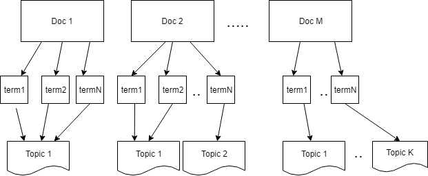
The input to the algorithm is a document-term matrix. Where each topic consists of a set of words where order doesn’t matter, So it is a Bag Of Word implementation.
We have two assumptions for Topic Modelling Algorithms that we are going to discuss,
- each document consists of a mixture of topics
- each topic consists of a collection of words
LSA: Latent Semantic Analysis
In this, we generate a matrix $ A^{ m \times n }$ where m is the number of documents and n is the number of words or terms. So each row represents a document and each column represents a word. Each cell has a raw count of the appearance of the word but the better solution is to have a tf-idf score of that word. and tf-idf is \(w_{i,j} = tf_{i,j} \times \log \frac{N}{df_{j}}\)
Where $ w_i,j $ is the tf-idf score. $ tf_{i,j} $ Number of occurrences of term in document $ N $ Total Documents $ df_{j} $ Number of documents containing words Once we have A we can start thinking about latent topics but the problem is that A is a very large, sparse and noisy matrix. To perform computation we will have to use Dimensionality Reduction. Let’s use truncated SVD for that. (More on SVD later or you can study using google )
So, \(A = U_{t}S_{t}V_{t}^{T}\) where $ U_t \in \mathbb{R}^{m \times t} $ is document-topic matrix and $ V_t \in \mathbb{R}^{m \times t} $ is a term-topic matrix. In $ U $ column represent $ t $ topics and row represents document vector of topics. In $ V $ column too represents $ t $ topics and row represents term vector of topics. Here $ t $ represents the truncated topics which are most significant dimentions in our transformed space.
With these documents, we can easily apply measures such as cosine similarities to evaluate.
- The similarity of different documents
- The similarity of different words
LSA is quick and easy to use but has few drawbacks
- lack of interpretable embeddings that is we don’t know whether the topics are arbitrary positive or negative
- We need huge datasets for it to perform well.
- less efficient representation
pLSA: Probabilistic Latent Semantic Analysis
pLSA is a Bayesian version of LSA. It uses Dirichlet priors for a document-topic and word-topic distribution. We assume how the text is generated is that you think of a topic and then for the words in that topic you pick a word and write it. The goal of this is to choose distributions such that the probability of the generation of the collection is MAX.
Okay So there is good math in this, let us talk about notations. $ d $ is document and $ w $ is word where $ d \in D $ and $ w \in W_d $ where $ D $ is number of documents and $ W_d $ is the word from the document d $ n_{wd} $ count of word in document d $ \phi_{wt} $ is the probability of the word in topic. $ \theta_{td} $ is the probability of the topic in that document.
According to the law of total probability, \(P(w) = \sum_{t \in T} P(w | t) P(t) \tag{1}\)
Similarly, \(pLSA = \sum_{t \in T} P(w | t,d) P(t|d) = \sum_{t \in T} P(w|t)P(t|d) \tag{2}\) This is an assumption we make and it is called as assumption of conditional Independence i.e $ P(w|t,d) = P(w|t) $ we don’t consider Probability of the word is dependent on the document, only dependent on topic.
We now will calculate the log likelihood and maximize its arguments: \(\log{\prod_{d \in D} p(d) \prod_{w \in d} P(w|d)^{n_{dw}} } \rightarrow \max{(\phi, \theta)}\)
Which is equal to \(\sum_{d \in D} \sum_{w \in d} n_{dw} \log{ \sum_{t \in T} \phi_{wt} \theta_{td} } \rightarrow \max{(\phi, \theta)}\)
We have normalized and non-negative constraints that means $ \phi_{wt} \geq 0 \ \& \ \theta_{td} \geq 0 $ Also, $ \sum_{w \in W} \phi_{wt} = 1 \ \& \ \sum_{t \in T} \theta_{td} = 1 $
So how it works, really… The Optimization generally used is E-M optimization. So we start with $$ P(t|d,w) = \frac{P(w| t,d)}{P(w|d)} = \frac{P(w|t)P(t|d)}{P(w|d)} $
The E step: \(P(t|d,w) = \frac{P(w|t)P(t|d)}{P(w|d)} = \frac{\phi_{wt} \theta_{td}}{ \sum_{s \in T} \phi_{ws} \theta_{sd} }\) The M Step: \(\phi_{wt} = \frac{n_{wt}}{\sum_w n_{wt}} \ \ \ \ n_{wt} = \sum_d n_{dw} P(t|w,d)\) \(\theta_{td} = \frac{n_{td}}{\sum_t n_{td}} \ \ \ \ n_{td} = \sum_W n_{dw} P(t|d,w)\)
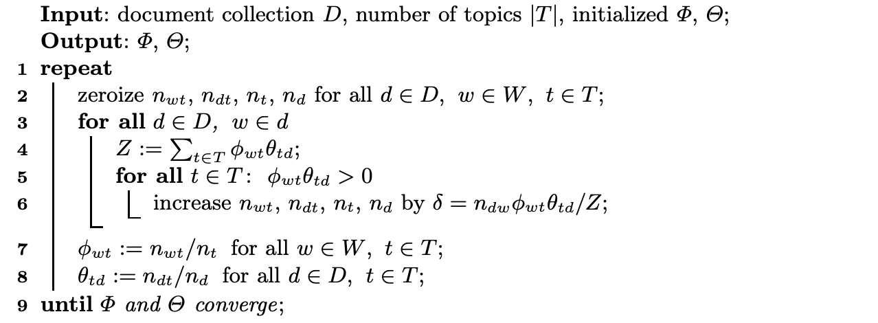
The Algorithm looks like this:
http://www.machinelearning.ru/wiki/images/1/1f/Voron14aist.pdf