
(Migrated from old blog)
We mentioned backpropagation in logistic regression and neural network, In that we used Gradient Descent and a fixed learning rate $\alpha $, for the method to go look for its steepest slope and start reducing towards the slope. But in that we have problems of overshooting and a fixed learning rate often have problem towards converging ( a terminology used to reach the minima).
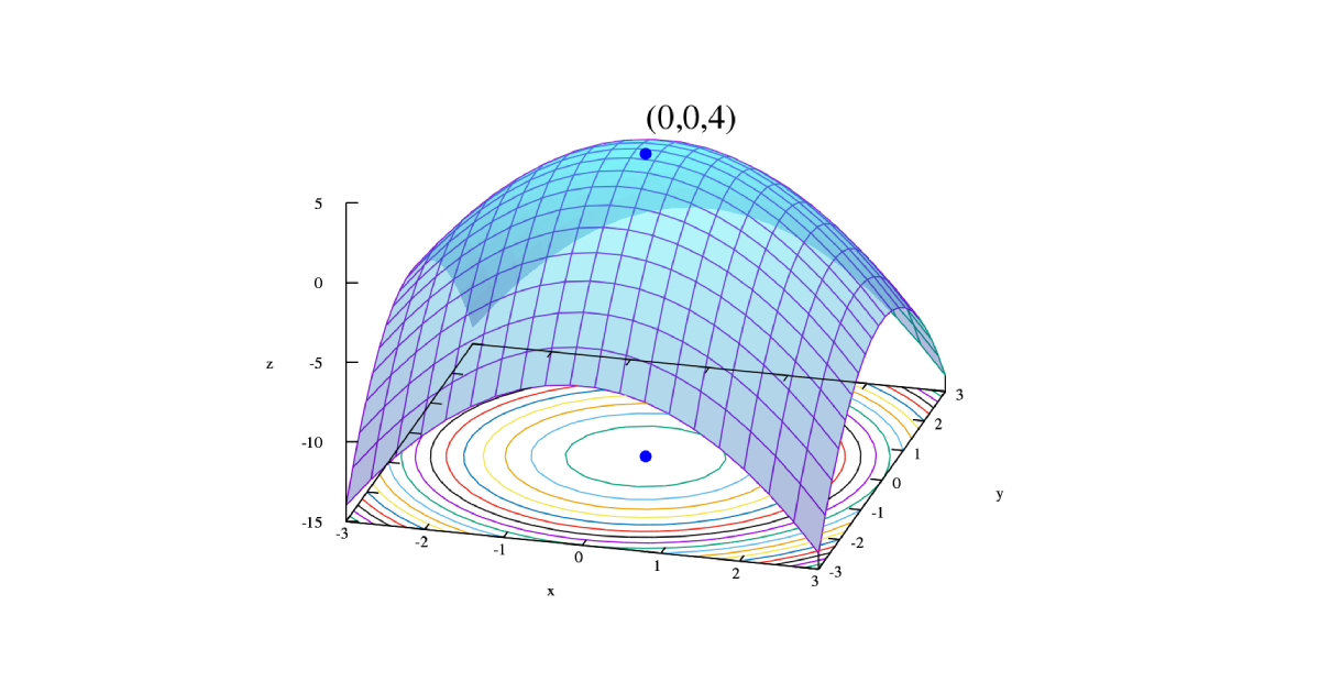
First Lets see some cool illustrations of how the optimization algorithms converge to the minima.
 Optimization algorithms and their convergence
We see in the end they all converge (mostly unless overshoots) but they all have different time where they all converge, some takes time some overshoots, some have adaptive learning rate, some has fixed, etc.
So lets talk about Gradient Descent First
Gradient Descent
We have been using it since the starting of this blog and didn’t mentioned its extensions until now, let’s do it.
The method remains the same in most of the optimization algorithms we calculate the loss function and start back propagation along with it.
In Gradient Descent we have a learning rate $\alpha$ which we set in the start, a good idea is to have an LR that is not too big to overshot and not converge and not too small to take a lot of steps to converge. So we usually check between, $\alpha = \left[ 0.1, 0.01, 0.001 \right] $ something like this. But it remains constant through the optimization process.
So we have a gradient value,
\[g_t = \frac{1}{n} \sum_{i=1}^{n} \nabla \mathscr{L} (x_i, y_i)\]And then we update the weights with the gradient and learning rate,
\[W^t = W^t - \alpha g_t \tag{1}\]Awesome, so that is how the gradient descent works for more details into its differentiation look at how the backpropagation works in Logistic regression post.
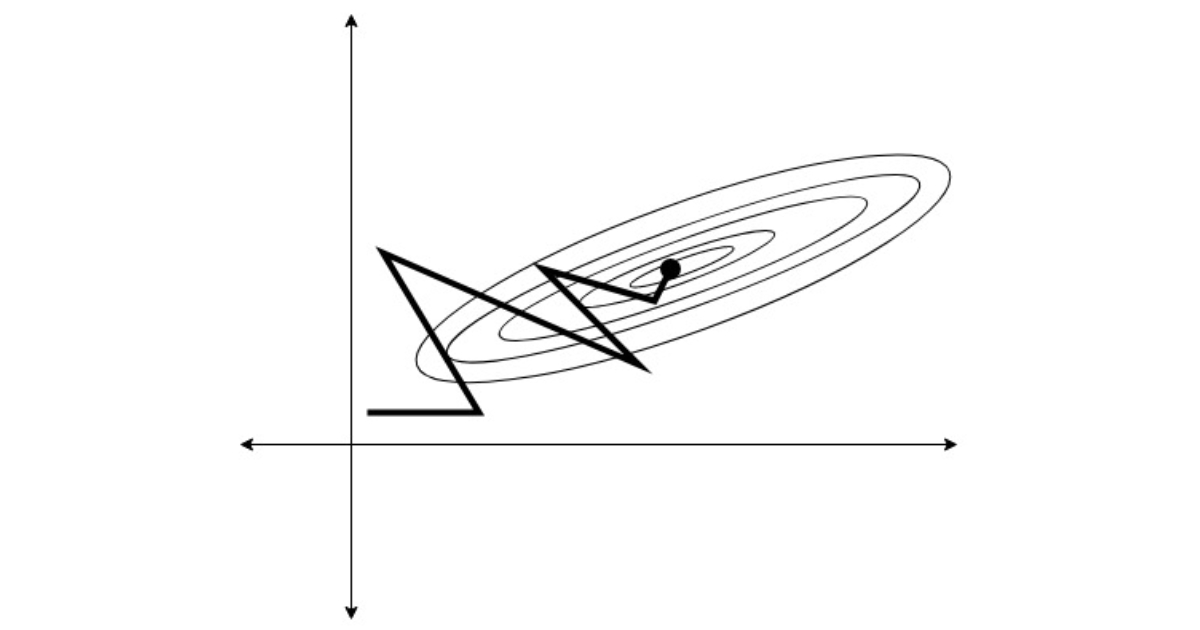
 Gradient descent
Mini Batch Gradient Descent
Instead of finding gradient of each and every training sample in the back-propagation progress we select m random samples and perform the gradient on only that mini batch, hence the name mini batch gradient descent.
Randomly initialize $W^0 $and repeat the process until the absolute difference of $W^t - W^{t-1} < \epsilon $where $\epsilon $is a very small value i.e when the gradients stop to change we can assume that we have converged and reached minima.
So for every iteration, we select M random samples from the training sample and find its gradient, $$ g_t = \dfrac{1}{m}\sum_{j=1}{m} \nabla \mathscr{L} (W^{t-1}_j, x_j, y_j ) $ Then approximate Gradients based on those m examples,
\[W^t = W^t-1 - \alpha g_t\]until
\[\vert\vert W^t - W^{t-1} \vert\vert < \epsilon\]Gradient Descent with Momentum
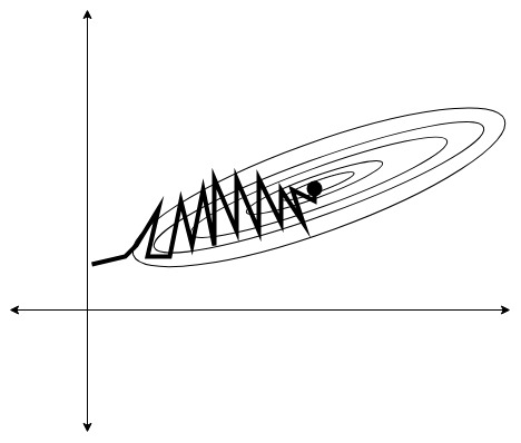
In this method, we maintain a $\textbf{h} $ state of all the steps for gradient descent and for next iteration, we take account of past value of $\textbf{h} $ and multiply it with some coefficient $\chi$ and then multiply the weights accordingly. Generally the value of $\chi = 0.9 $but we adjust as needed. But its a good value to start with, So the equation becomes
\[h_t = \chi h_{t-1} + \alpha g_t\]where $\alpha $is learning rate and $g_t $is the gradient of the whole process Now the weights are updated with the $h$
\[W^t = W^{t-1} - h_t\]Lets think why it works ? $h_t $ cancels some coordinates of the gradient that leads to oscillation of gradients i.e prevents overshooting by penalising the gradients for being too large , resulting in lesser oscillation and faster convergence.
 Gradient descent with momentum
Did you notice the lesser oscillations thus faster convergence ? Cool
Nestov Momentum
Extension to GD with momentum , in this we look at the direction of $h_t $and calculate some vector on the gradient of it and then take the gradient step with that.
So mathematically, it becomes,
\[h_t = \chi h_{t-1} + \alpha \nabla \mathscr{L} \left( W^{t-1} - \chi h_{t-1} \right)\]and update weights,
\[W^t = W^{t-1} - h_t\]It leads to better convergence and works with difficult functions with complete level sets.
But the method described above are very sensitive to learning rate as $\alpha $ remains constant in all of the above. Lets learn about Methods with adaptive learning rate
AdaGrad
Adaptive Gradient or AdaGrad, in this the learning rate is adaptive.
We take the Gth coordinator of parameter vector W and to make a gradient step we take jth component of parameter vector from previous iteration i.e $W_j^{t-1} $and subtract jth component of the gradient of current point, to find out the next parameter approximation of $W^t_j $.
We use $G $, we take $G_j^{t-1} $and we add the square of gradient at the current iteration. So mathematically,
$$ G_j^t = G_j^{t-1} + g^2_{t_j} $where $G $is sum of square of gradients of all the previous iterations and then update the weight as
\[W_j^t = W_j^{t-1} + \dfrac{\alpha}{\sqrt{G_j^t + \epsilon}} g_{t_j}\]where $\epsilon $is a very small value to prevent division by zero
Pros:
- This method then chooses lr adaptively, initialize by setting a lr like 0.01 and it will auto adapt based on gradients to converge better.
- Useful for sparse data
- Separate learning rate for each dimension
- $G_j^t $always increases, leads to early stopping.
Cons:
Sometimes $G $becomes too large that the gradient descent will stop building
RMSProp
To overcome the con of adagrad i.e large sum of square of gradients we add something like momentum to calculation of $G $i.e to calculate $G^t_j $at some step t we take $G_{j}^{t-1} $from previous step t-1
\[G^t_j = \chi G^{t-1}_j + \left( 1- \chi \right) g^2_{t_j}\]again $\chi \approx 0.9 $ generally
And then we update weights as
\[W^t = W^{t-1} + \dfrac{\alpha}{\sqrt{G_j^t + \epsilon}}g_{t_j}\]LR adapts to the latest gradient and overcomes large sum of square problem but it is little biased towards zero because we initialize it with zeroes.
Adam Optimizer
It calculates exponentially weighted sum of gradients from all iterations, we take $V^t $from previous step $V_j^{t-1} $.
So to overcome biasing of RMS we do,
\[V_j^{t} = \dfrac{ \beta_2V^{t-1} + \left( 1 - \beta_2 g^2_{t_j} \right) }{ 1 - \beta_2^t }\]This normalization allows us to get rid of bias present, now we update weight as
\[W^t_j = W^{t-1}_j - \dfrac{\alpha}{\sqrt{V_j} + \epsilon} g_{t_j}\]But, the gradient can be noisy so we maintain another auxiliary variable $m $that is the sum of gradients as smoothening variable. So Mathematically, the final optimization becomes,
\[m_j^t = \dfrac{\beta_1 m_j^{t-1} + \left( 1 - \beta_1 \right) g_{t_j} }{ 1 - \beta_1^t}\]this is the sum of all gradients till time t.
\[V_j^t = \dfrac{\beta_2 V_j^{t-1} + \left(1 - \beta_2 \right) g_{t_j}^2 } {1 - \beta_2^t}\]this is the sum of square of all gradients till time t
Final Weight update as
\[W^t_j = W^{t-1}_j - \dfrac{\alpha}{\sqrt{V_j} + \epsilon} m_{t_j}\]This Converges way better and faster than other algorithms mostly.