A beginners guide to SVM

(Migrated from old blog)

One of the method of optimization that sometimes yield good results are is widely used in Support Vector Machines

Optimization Objective

First, Let’s read a little about logistic regression and its loss function and modify the loss function

Read About Logistic Regression And Its Loss Function Here

So the loss function for logistic regression is

\[\underset{\theta}{\mathrm{max}} \frac{1}{m} \sum_{i=1}^{m} – ( y^{(i)} \log h_\theta(x) + (1-y^{(i)}) \log (1 – h_\theta( 1- y^{(i)}) + \frac{\lambda}{2m} \sum_{j=1}^{m} \theta^2_j\]

with the regularization parameter $\lambda $, we can write the equation as $-( \log h_\theta(x) ) = \mathrm{Cost}_1(\theta^T x) $ i.e when y= 1 and the cost of the function is return with the parameter $\theta^T x $ from the sigmoid function $\frac{1}{1 + e^{-\theta^Tx}} $ .

So the whole equation become,

\[\underset{\theta}{\mathrm{max}} \frac{1}{m} \sum_{i=1}^{m} ( y^{(i)} \mathrm{Cost}_1(\theta^T x) + (1-y^{(i)}) \mathrm{Cost}_0(\theta^T x) + \frac{\lambda}{2m} \sum_{j=1}^{m} \theta^2_j\]

Now we can remove some constants as they will not help in minimising out objective argument $\theta $ and put $C = \frac{1}{\lambda} $

The Equation becomes :

\[\min_{\theta} C \sum_{i=1}^{m}\left[y^{(i)} \mathrm{cost}_{1}\left(\theta^{T} x^{(i)}\right)+\left(1-y^{(i)}\right) \mathrm{cost}_{0}\left(\theta^{T} x^{(i)}\right)\right]+\frac{1}{2} \sum_{i=1}^{n} \theta_{j}^{2}\]

This equation can be represented as $CA+B $ and the hypothesis becomes

\[h_\theta (x) = \begin{cases} 1 & \text{if } \theta^T \geq 0 \\ 0 & otherwise \end{cases}\]

Lets , Look at the graph of $\mathrm{Cost}_0 $ and $\mathrm{Cost}_1 $

Cost Method of Cost 1 and Cost 0 of the SVM cost functions : from Master AndrewNG

Now SVM doesn’t only says that $y = 1 $ when $\theta^T x \geq 1 $ not just 0 similarly, when $y= 0 $ when $\theta^T x \leq -1 $ not just 0 which gives an extra safety margin in SVM over logistic regression.

So, If the value of $C $ is very large we will want to set the first equation of $CA +B $ i.e $A $ equal to $0 $ to minimise the equation as C is in multiplication. So the Large Margin Classifier Minimization function becomes

\[\min_\theta \frac{1}{2} \sum_{j=1}^{n} \theta^2_j\]

when

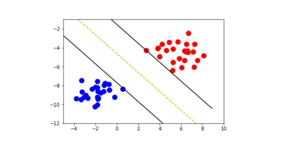
\[\begin{aligned} \text { s.t. } & \theta^{T} x^{(i)} \geq 1 & \quad \text { if } y^{(i)}=1 \\ & \theta^{T} x^{(i)} \leq-1 & \quad \text { if } y^{(i)}=0 \end{aligned}\]

In SVM we maximize margin between two datasets

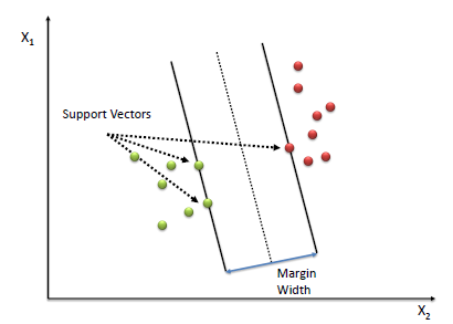Support Vector Machines showing the Margin width and support vectors

The goal is to maximise margin width with that loss function which is

\[\min_\theta \frac{1}{2} \sum_{j=1}^{n} \theta^2_j = \min_\theta \frac{1}{2} \sum_{j=1}^{n} \vert \vert \theta\vert \vert _j \tag{1}\]

which means the norm of theta i.e $\vert \vert \theta \vert \vert = \theta^2$ has to be minimised and the hypothesis now becomes that by Vector Algebra we know that scalar product of two vectors $\vec{u} $ and $\vec{v} = u^Tv = P.\vert \vert u\vert \vert $ where $P $ is the project of $\vec{u} $ on vector $\vec{v} $.

So the Hypothesis becomes :

\[\begin{cases} P^{(i)} \vert \vert \theta\vert \vert >1 & if y^{(i)} = 1 \\ P^{(i)} \vert \vert \theta \vert \vert < -1 & if y^{(i)} = 0 \end{cases}$ where $P^{(i)}\]

is the projection of $x^{(i)} $ onto vector $\vec{\theta} $

How SVM Maximises the boundaries

First, we need to understand that to maximize the margin the normal to the vector should be the boundary and the sum of the project of the vectors on either side of the boundary should be maximum. Assumption $\theta_0 = 0 $

Therefore, Consider the case of margin where

SVM with a non optimal margin

Here green line is the normal to the vector $\vec{\theta} $ and AO is the projection of $x^{(1)} $ on vector $\vec{\theta} $ , as $P^{(1)} $ for the case $y = 1 $ we know that $P^{(i)} \vert \vert \theta \vert \vert \geq 1 $. Also we use for case $y = 0 $ where BO is the projection of $x^{(2)} $ for this $P^{(i)} \vert \vert \theta \vert \vert \leq -1 $.

But in these cases the value of $P(^{(i)} $ will be very small so in order to meet condition like $P^{(i)} \vert \vert \theta \vert \vert \geq 1 $ and $P^{(i)} \vert \vert \theta \vert \vert \leq 1 $ the $\vert \vert \theta \vert \vert $ has to be very large. but the objective of the minimization function check equation (1) is to minimize norm of $\theta $. Therefore, it is not an ideal condition and SVM will not choose this decision boundary.

Now consider the case where SVM chooses decision boundary as :

SVM Optimally dividing the two classes

So now the SVM chooses green line and Vector $\theta $ is the vector and again AO and BO are projection of datasets $x^{(1)} $ and $x^{(2)} $, now the value of projections $P^{(1)} $ and $P^{(2)} $ for cases $P^{(i)} \vert \vert \theta \vert \vert \geq 1 $ and $P^{(i)} \vert \vert \theta \vert \vert \leq 1 $ respectively is much bigger now this condition can hold true even when norm of $\theta^2 $ is smaller.

Therefore the SVM will chose the second hypothesis than the first one and this is how SVM gives the large margin classifier.

Read about Kernels here : Before continuing

Kernels

So, now the hypothesis becomes , Given: $x $ compute features, $f \in \mathbb{R}^{m+1} $ Predict $y=1 $ if $\theta^Tf \geq 0 $

Training Algorithm :

\[\min_{\theta} C \sum_{i=1}^{m}\left[y^{(i)} \mathrm{cost}_{1}\left(\theta^{T} f^{(i)}\right)+\left(1-y^{(i)}\right) \mathrm{cost}_{0}\left(\theta^{T} f^{(i)}\right)\right]+\frac{1}{2} \sum_{i=1}^{n} \theta_{j}^{2}\]

About the Parameter $C = \frac{1}{\lambda} $ Large Value of C : Lower bias , High Variance Smaller Value of C : Higher Bais, Lower Variance

Parameter $\sigma^2 $ Large Value of $\sigma^2 $ : feature $f_i $ varies more smoothly. Higher bais, Lower Variance Small Value of $\sigma^2 $ : feature $f_i $ varies more abruptly. Lower bais, Higher Variance

When to use what Kernel :

• Linear Kernel: Linear Kernel or no kernel is used when you don’t have enough training data set and a large list of features, in that scenario we need not fit a complex equation just a linear decision boundary should be enough to fit it.
• Gaussian Kernel: It should be used when the list of features is small and the dataset is pretty large, the kernel will help to fit complex non-linear boundary. or any Other Kernel.