
(Migrated from old blog)
To understand about this topic you should ideally read this post about neural networks and its formulas because I will be continuing from there so first check out this link about Neural Networks.
So the details for gradient descent was mentioned in the post where we talked about logistic regression with a neural network approach. I will recommend you to read gradient descent from here as it will have more explanation than this post. But let me try with this post too.
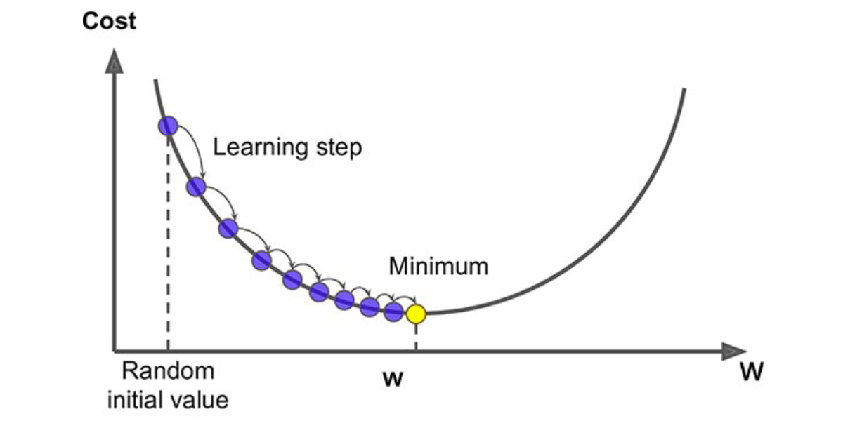
Gradient descent is an optimization algorithm used to minimize some function by iteratively moving in the direction of steepest descent as defined by the negative of the gradient. In machine learning, we use gradient descent to update the parameters of our model. Parameters refer to coefficients in Linear Regression and weights in neural networks.
https://ml-cheatsheet.readthedocs.io/en/latest/gradient_descent.html
So basically, gradient descent is an optimization algorithm where you minimize the loss function by taking the derivative of the loss function and finding the arguments (weights ) for which the loss function is minimal. Enough of English, Lets talk Math now.
Let’s write the equations for forward propagation that we know for neural networks,
\[z^{[1]} = W^{[1]} X + b^{[1]}\]where Dimentions of $ W^{[1]}$ is $\left( n^{[1]} \times n^{[0]} \right)$ where the number represent the layer of the network therefore $ n^{[0]} $ is the size of input. Similarly, Dimentions of $ b^{[1]}$ will be $ \left( n^{[1]} \times 1 \right) $ Next Equation,
\[A^{[1]} = g^{[1]}(z^{[1]})\]where $ g^{[1]}$ is any activation function we talked about in neural network post.
Then, \(z^{[2]} = W^{[2]} X + b^{[2]}\)
where Dimentions of $ W^{[2]}$ is $ \left( n^{[2]} \times n^{[1]} \right)$ and dimentions of $ b^{[2]}$will be $ \left( n^{[2]} \times 1 \right) $ and
\[A^{[2]} = g^{[2]}(z^{[2]})\]Perfect, now let’s start about the backward propagation, I will not try to reinvent the wheell. So if you don’t know what backward propagation is, I will recommend you to watch this video from 3Blue1Brown which I think is one of the best and simplest explanation of backward propagation.
3Blue1Brown video on backpropagation
Lets assume after all the forward propagation we found the predictions as $Y$ So backpropagations begins like ,
\[dz^{[2]} = A^{[2]} - Y\]And,
\[dW^{[2]} = \frac{1}{m} dz^{[2]} A^{[1]T}\]Similar to logistic regression,
\[db = \frac{1}{m} np.sum(dz^{[2]}, axis=1, keepdims=True)\]where np.sum is a numpy command to sum the whole array and keep the dimensions the same that were input along the y axis. Furthur backpropagation we get,
where $g’$ is a derivative of the activation function and $*$ is the element wise product. And Finally,
\[dW^{[1]} = \frac{1}{m} dz^{[1]} X^T\]and
\[db = \frac{1}{m} \text{np.sum}(dz^{[1]}, \text{axis}=1, \text{keepdims}=True)\]Here is a summary of gradient descent by Andrew NG and I think its the best to sum up Gradient Descent

Summary of Gradient Descent
A programmatical Implementation of this can be found in my repository : https://github.com/shivammehta25/NLPResearch/blob/master/Tutorials/NeuralNet/Neural%20Network%20From%20Scratch.ipynb.