

(Migrated from old blog)
If your dataset is overtrained i.e it has high variance then one of the possible ways to reduce that is either to get more training data which sometimes can be very costly, or one of the approach is regularisation.
Regularization: It is a form of regression where we force the coefficients to reduce/shrink estimates to zero. It is the form of discouraging the learning to learn too much on complex data so as to overfit model with that data.
Lets begin with regularizing the logistic regression loss function
\[J_{w,b} = \frac{1}{m} \sum_{i=1}^{m} L(\hat{y}^{(i)}, y^{(i)})\]where
\[w \in \mathbb{R}^{n_x} \ and \ b \in \mathbb{R}\]as the weights and biases.Now, In order to regularize it all we have to do is add normalization of $ \vert\vert w\vert\vert_2^2 $ with a regularization parameter $ ( \lambda) $ so the final equation becomes
\[J_{w,b} = \frac{1}{m} \sum_{i=1}^{m} L(\hat{y}^{(i)}, y^{(i)}) + \frac{\lambda}{2m} \vert \vert w\vert \vert ^2_2\]where $ \vert\vert w\vert\vert_2^2 = \sum_{j=1}^{n_x} w_j^2 = w^Tw $
This is also known as L2 Regularization or Ridge Regularization. It is the most common form of regularization.
Another Type of regularization is L1 regularization or Lasso Regularization we just add
\[\frac{\lambda}{2m} \vert\vert w\vert\vert_1 = \frac{\lambda}{2m} \sum_{j=0}^{n_x} \vert w_j\vert\]It is also known as lasso regularization.
This is less commonly used but is used to reduce the space as it generates a lot of sparse vectors. How? Let’s see,
We can say that the L1 regularization is the solution of the equation where the sum of modulus of each coefficient is less than the value s which is a constant value that exists for all values of shrinkage factor aka $ \lambda (lambda) $. Similarly, L2 regularization is the sum of squares of coefficients.
Consider only 2 parameters so the coffiecients comes for L1 regularization as
\[\vert w_1\vert + \vert w_2\vert \leq s \tag{1}\]and for L2 it becomes
\[w_1^2 + w_2^2 \leq s \tag{2}\]By looking at these equations we can see that equation (1) is an equation of rectangle while the equation (2) is the equation of square. So we can depict it as
 L1 and L2 Regularization: Credit : An Introduction to Statistical Learning by Gareth James, Daniela Witten, Trevor Hastie, Robert Tibshirani
Left is L1 and Right is L2 and the eliptical path is RSS. The values of the coefficient are determined by the point of contact between the green area and the red ellipse. Since L2 has a circular parameter the contact will not occur generally at any specific axis, while for the L1 it is rectangular and the contact will generally occur at axises therefore, when it will occur one of the coefficients will become zero. Same thing in higher dimention will yield lot of zeroes in the Weight matrix, thereby generating a sparse matrix.
So, what is lambda ? $ \lambda $. Lambda is the regularization parameter and is just another hyperparameter that we will have to tune. Usually we set this using the development set along with other hyperparameter tuning, or during cross validation.
So this was the case for Logistic Regression. Let’s talk about Neural Networks
Neural Network
Similarly, like the case of Logistic regression for Neural network, we know the loss function as
\[J(w^{(1)}, b^{(1)}, ... , w^{(l)}, b^{(l)}) = \dfrac{1}{m} \sum_{i=0}^{m} L(\hat{y}^{(i)}, y^{(i)})\]we can regularize it by adding a regularization factor which makes it as
\[J(w^{(l)}, b^{(l)}) = \dfrac{1}{m} \sum_{i=0}^{m} L(\hat{y}^{(i)}, y^{(i)}) + \dfrac{\lambda}{2m} \vert \vert w^{[l]}\vert \vert ^2_F\]Where $ \vert\vert w^[l] \vert \vert ^2 $ is Frobenius Normalization also denoted as $ \vert \vert \cdot \vert \vert_2^2 \ or \ \vert \vert \cdot \vert \vert ^2_F $.
Applying it into the backpropagation our equations have a little change even though the derivative wrt the variables doesnot changes just a little change in weights is seen. i.e called as weight decay. So the equation becomes,
\[dw=\text{value from back propagation} + \dfrac{\lambda}{m} W^{[l]}\]and
\[W^{[l]} = W^{[l]} - dw\] \[W^{[l]} = W^{[l]} - \alpha \left[ \text{ value from back propagation } + \dfrac{\lambda}{m} W^{[l]} \right]\]Where
\[W^{[l]} = W^{[l]} \left( 1 - \dfrac{\lambda}{m} \right) - \alpha \text{value from back propagation}\]Since the weights is getting reduced by $ \dfrac{\lambda}{m} $ therefore it is also known as weight decay.
Dropout Regularization
Dropout is a strange way of regularization just at any probability you start dropping out random number of elements from a neural network layer. Dropping out means, you ignore those nodes and do not use them for backpropagation calculation and forward propagation calculation. This adds a randomness to the network and everytime you train a smaller network, which prevents over fitting.
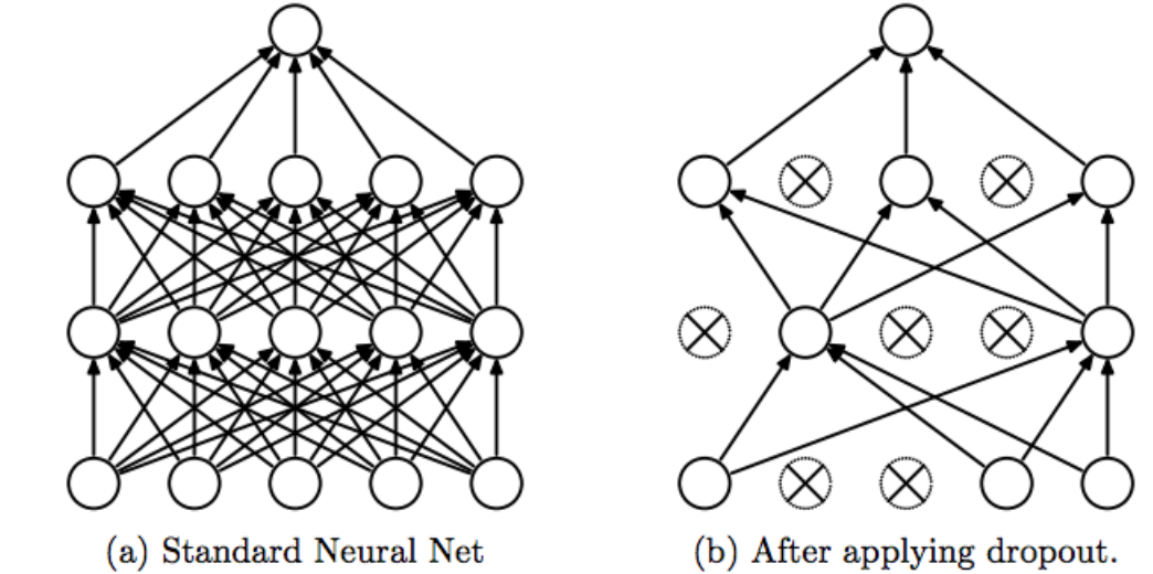 Dropout Regularization
Inverted Dropout
One of the way of implementing the dropout is inverted dropout. In Inverted Dropout you randomly dropout the neurons with $ p $ dropout rate and so as to not to return the diminished value to the next layer we multiply the activation by a factor of $ \dfrac{1}{p} $ where $ p < 1 $ and thus it will increase the multiplier and hence the activations will be managed. So lets see how it works in code
Lets Assume for a layer 3 we are applying dropout we will write it as
1
2
3
4
5
keep_prob = 0.8
d3 = np.random.rand(*a3.shape) < keep_prob
a3 = np.multiply(a3, d3)
a3 /= p #This is the Inversion Step called as inverted dropout technique
z4 = np.dot(W4, a3) + b4
Some Other Regularization Technique
Data Augmentation
As we read on the machine learning post that Data Augmentation means generating more data from the previous data present, generally done in Computer Vision tasks where the image is flipped, rotated and random crops of the image is used as long as it makes sense and additional data is generated for the model to learn and train on.
Early Stopping
In early stopping you will plot the train set error and at the same time use the dev set error plotting too, and generally the dev set error will decrease till some time and then will start to increase monotonically, So we stop the neural network training in the halfway where the dev set error is the minimum. It breaks the orthogonoalization (First finding the minimum cost function and then preventing overfitting). The better approach is to use L2 regularization the only downside to L2 reguarization is the computation of the extra hyperparameter $ \lambda $ (lambda).