Machine Learning Theory

(Migrated from old blog)

We will talk about a lot of theory in this post. So,

• Machine Learning: A machine is said to be learning when with some E experience with respect to some task T and some performance measure P and it improves performance P on the task T with experience E.

• Weak AI: A computer system which computes and performs intelligent computations based on the algorithm and codes coded into the system. It is based on the theory that instead of converting computers into humans we should ask them to do complicated tasks with the information provided to them and compute the results. The tasks are entered manually. Example: automatic car or remote control devices.

• Strong AI: This a new type of technology that tries to mimic a human mind and take a decision on its own. The main advantage of this technology is that no human intervention is required, the machine is capable enough to process data and take the decision based on the data. Example ChatBots.

Supervised Learning: In supervised learning, the algorithm learns from labeled data. It first understands the data and after understanding the data it formulates what should be done with the new data based on the labels and patterns in the training dataset. Supervised Learning can be categorized into two different types:

Classification: Technique used to determine in which of the following category the data belongs to. A classifier understands the training data in which class the input data belongs to. Example of classification problems includes spam detection, sentimental analysis, etc.

Regression: Technique, where a model is devised from the data and the prediction, is made on the basis of the model’s result. The model is devised by measuring the relationship between variables and the output is predicted with the help of that mathematical model.

Learning Method: It is a mapping $ \mu : (X \times Y)^{\ell} \rightarrow A $ which returns an algorithm $ a \in A $ for a given training set $ T^{\ell} $. It consists of two steps :

Training Step: In which you build a model $ a $ from training set $ T^{\ell} \ \Rightarrow a = \mu(T^{\ell}) $.

Testing Step: In this you predict the new dataset (x) with the help of a $ a(x) $

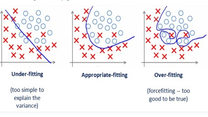
Overfitting vs Underfitting vs Appropriate Fitting

• Overtiftting and Underfitting:

  • Overfitting: When the model is too tightly fitted on your dataset, it tend to overperform and fits even outliners and noise. This result in poor results when tried with the testing dataset. $ (T^{\ell}) $. These are also called High Variance.
    • We use regularization to overcome the problem of Overfitting. Types of Regularization
      • L1 Regularization / Lasso Regularization: Least absolute shrinkage and selection operator, a penalty $P = \alpha \sum_{n=1}^{N} \vert \theta_n \vert$ is added to every minimization, which reduces any terms to zero if they are irrelevant which results in dimensionality reduction and used in feature selection as well.
      • L2 Regularzation / Ridge Regularization: In this $ P = \alpha \sum_{n=1}^{N} \theta_n^2 $ term is added but instead of reducing the irrelevant term to zero it reduces its values.It will not get rid of the features but will rather reduce its effect on the model.
      • Elastic: It is the combination of both L1 regularization and L2 Regularization thus it results the best results the term that is added is : $ P = \alpha \sum_{n=1}^{N} \vert \theta_n \vert + (1 - \alpha) \sum_{n=1}^{N} \theta_n^2 $
  • UnderFitting: More on this later.
• Validation: We divide the dataset into three sets, one is the train, test, and validation. We train the model using training dataset and then tune the hyperparameters in the validation dataset. Once the model is fine-tuned in validation dataset we use those values of hyperparameters to test the model in the testing set.
• Cross-Validation: In this, we split the dataset $ (\ell) $ into two sets, one is training test $ (T^{t}) $ and the other is testing set $ (T^{\ell-t}) $. We train the model into the training test and then do testing and accuracy calculation based on the results of the testing set.
• K-Fold Cross Validation: In this, the dataset is split into k sets (folds) and each set is a testing set once. So it is repeated for k folds where one part is a testing set rest others are all training sets on which the model is trained.
• Leave One Out Cross Validation: In this, we split the dataset into $ \ell - 1 $ and $ 1 $ value. For each iteration, we have just 1 value as testing set or value. We iterate from the starting value to the last in the dataset and calculate measures based on those results.

Accuracy, Recall, Precision: For this, we need to first understand what is let’s assume we have a confusion matrix:

	Predicted Negative	Predicted Positive
Actual Negative	True Negative	False Positive
Actual Positive	False Negative	True Positive

Let’s assume our classifier or model is a binary classifier which gives either correct or incorrect value ( given positive and negative respectively). The measures for such can be calculated as

• Precision: It tells of how many positives does the classifier predicted, i.e the ratio of true positive with all the predicted positive’s: i.e$ Precision = \frac{\text{True Positive}}{\text{True Positive} + \text {False Positive}}$

• Recall: It tells us how many were actually positive, i.e the ratio of True Positive with all the actual postive’s i.e :\(Recall = \frac{\text{True Positive}}{\text{True Positive} + \text {False Negative}}\)

• Accuracy: It is the total number of correct predictions i.e the ratio of true negative and true positive with the total number of samples i.e$ Accuracy = \frac{\text{True Positive} + \text{True Negative}}{\text{True Positive} + \text {False Negative}+ \text{True Negative} + \text{False Positive}}$

• F1 Score: It is a better measure than Accuracy it is a balance between the Precision and Recall. Also when there is uneven class distribution ( or large number of true negative’s) F1 Measure is calculated by :\(F1 Score = 2 \times \frac{Precision * Recall} {Precision + Recall}\)

• Mean Absolute Error: It measues the error in the prediction without considering the differences of direction. It is the average over the absolute difference between the predicted and actual value. It is usefull but sometimes it can be faulty as it cancels the negative and positive errors. \(MAE = \frac{1}{n} \sum_{i=1}^{n} \vert X_i - \hat{X_i}\)

• Mean Square Error: It is the measure of the average magnitude of the error. But it gives bigger value for weights because of the squaring of the differences. It is very useful when the large values are undesirable. \(MSE = \frac{1}{n} \sum_{i=1}^{n} (X_i - \hat{X_i} )^2\)

• Batch gradient descent: In Batch gradient descent, we find the minimisation of the cost function by differentiating each and every value in the dataset. This can be a heavy operation but path to minima is less noisier. $ \theta_j = \theta_j - \alpha \frac{d J(\theta)}{d\theta} $ where $ \frac{d J(\theta)}{d\theta} = \frac{1}{m} \sum_{i=0}^{m} \vert y_i - \hat{y}_i \vert $ or any distance function.

• Stochastic Gradient Descent: Instead of finding the cost function of each and every value we just use a random value and minimize it in every iteration. This is a comparatively lighter operation and is used more often than Batch Gradient Descent. The path to minima is noisier.$ \theta_j = \theta_j - \alpha $ where $ \alpha = \vert y_i - \hat{y}_i \vert $ or any other distance function.

• Linear Regression: Detailed Post Later but for now, Linear Regression is used to find the relationship between two or more variables, the core idea is to fit a line $ y = \theta_0X + \theta_1 $ for which the error is minimum. It is used in the predictive analysis. Generally, we reduce the mean square error or gradient descent. Generally Error is mean square error $ Error = \sum_{i=1}^n (\text{Predicted} - \text{Actual Output})^2 $ we minimise this.

  • Ridge Regression: ( L2 Regularization) A penalty is added which the sum of the square of all the magnitudes of the equation.$ Error = \sum_{i=1}^n (\text{Predicted} - \text{Actual Output})^2 + \lambda \sum_{i=0}^{n} \theta_i^2 $. So the ridge term (lambda) penalizes if the weights become large enough. So it shirings the coefficients and helps to reduce the model complexity and multi collinearity. ( Doesn’t turns them to zero)
  • Lasso Regression: Like ridge in Lasso a penalty is added to the error function but instead of the square of weight an absolute value is added.$ Error = \sum_{i=1}^n (\text{Predicted} - \text{Actual Output})^2 + \lambda \sum_{i=0}^{n} \vert\theta_i\vert $. This can lead to zero coefficients and is very usefull in feature selection.