

(Migrated from old blog)
I will recommend you first read my post about regularization here :
Regularization in Neural Networks
So we are done with basics of regularization we know we will add something like weight decay, but why do we add. Lets Discuss this,
Suppose we have set of instances $ x_i, y_i $ of a true model $ f_0 $ the instance can be test or training set and the output will be mapped with the equation and noise $ \varepsilon_0 $
\[y_i = f_0 + \varepsilon_0\]where $ f_0 $$
is a function mapped where input is $ x_i $
We develop a neural network and generate an estimator model $ \widehat{f_0} $
The Mean Squared Error can be calcualted as
\[\mathbb{E}\left(\left(\widehat{f_{0}}-y_{0}\right)^{2}\right) = \mathbb{E}\left(\left(\widehat{f_{0}}-f_{0}-\varepsilon_{0}\right)^{2}\right)\] \[=\mathbb{E}\left(\left(\hat{f_{0}}-f_{0}\right)^{2}+\varepsilon_{0}^{2}-2 \varepsilon_{0}\left(\widehat{f_{0}}-f_{0}\right)\right)\] \[=\mathbb{E}\left(\left(\widehat{f}_{0}-f_{0}\right)^{2}\right)+\mathbb{E}\left(\varepsilon_{0}^{2}\right)-2 \mathbb{E}\left(\varepsilon_{0}\left(\widehat{f}_{0}-f_{0}\right)\right)\] \[= \mathbb{E}\left(\left(\widehat{f}_{0}-f_{0}\right)^{2}\right)+\sigma^{2}-2 \mathbb{E}\left(\varepsilon_{0}\left(\widehat{f}_{0}-f_{0}\right)\right) \tag{1}\]The Last term is
\[\mathbb{E}\left(\varepsilon_{0}\left(\widehat{f}{0}-f{0}\right)\right) = \mathbb{E}\left(\left(y_{0}-f_{0}\right)\left(\widehat{f_{0}}-f_{0}\right)\right) \tag{2}\]To calculate this we use instances $ x_0, y_0 $
For instance instance $ x_0 , y_0 $ , there can be two possibilities
- The instance is not in training set
- The instance is in training set
Case I : The instance is not in training set
The Equation (2) becomes zero as
\[\mathbb{E}\left(\left(y_{0}-f_{0}\right)\right)=\mathbb{E}\left(y_{0}\right)-\mathbb{E}\left(f_{0}\right) \stackrel{(c)}{=} f_{0}-f_{0}=0\]And Equation (1) becomes
\[\mathbb{E}\left(\left(\widehat{f_{0}}-y_{0}\right)^{2}\right)=\mathbb{E}\left(\left(\widehat{f_{0}}-f_{0}\right)^{2}\right)+\sigma^{2}\]For lets say $ m $ instances the term will become
\[\sum_{i=1}^{m}\left(\widehat{f}_{i}-y_{i}\right)^{2}=\sum_{i=1}^{m}\left(\widehat{f}_{0}-f_{0}\right)^{2}+\underbrace{\sum_{i=1}^{m} \sigma^{2}}_{=m \sigma^{2}}\]Thus the error becomes,
\[\textbf{ Emperical Error }=\textbf { True Error }+m \sigma^{2}\]Therefore, in this case the emperical error is a good estimation of the true error.
Case II : The instance is in training set
To calculate this we will use Stein’s Unbiased Risk Estimator Lemma. That says that for a Multivariate Random Variable, $ \mathbb{R}^d \ni z = \left[z_{1}, \dots, z_{d}\right]^{\top}$ whose components are variables with normal distribution, i.e $ z_i \sim N(0,\sigma) $ . We take $ \mathbb{R}^d \ni \mu = [\mu_1, \dots, \mu_d]^\top $ and let $ \mathbb{R}^d \ni g(z) = [g_1, \dots, g_d]^\top $ be a function of random variable $ z $ with $ g(z) : \mathbb{R}^d \rightarrow \mathbb{R}^d $ There exists a lemma known as Stein’s Lemma
\[\mathbb{E}\left((\boldsymbol{z}-\boldsymbol{\mu})^{\top} \boldsymbol{g}(\boldsymbol{z})\right)=\sigma^{2} \sum_{i=1}^{d} \mathbb{E}\left(\frac{\partial g_{i}}{\partial z_{i}}\right)\]Now the Equation (2) Can be written as
\[\mathbb{E}\left(\left(y_{0}-f_{0}\right)\left(\widehat{f_{0}}-f_{0}\right)\right) = \sigma^{2} \mathbb{E}\left(\frac{\partial\left(\widehat{f_{0}}-f_{0}\right)}{\partial \varepsilon_{0}}\right)\] \[=\sigma^{2} \mathbb{E}\left(\frac{\partial \widehat{f}_{0}}{\partial \varepsilon_{0}}-\frac{\partial f_{0}}{\partial \varepsilon_{0}}\right) {=} \sigma^{2} \mathbb{E}\left(\frac{\partial \widehat{f}_{0}}{\partial \varepsilon_{0}}\right)\]Since $ \frac{\partial f_0}{\partial \varepsilon_0}$ is independent of noise.
\[{=} \sigma^{2} \mathbb{E}\left(\frac{\partial \widehat{f_{0}}}{\partial y_{0}} \times \frac{\partial y_{0}}{\partial \varepsilon_{0}}\right) {=} \sigma^{2} \mathbb{E}\left(\frac{\partial \widehat{f_{0}}}{\partial y_{0}}\right)\]Since $ y_0 = f_0 + \varepsilon_0 \rightarrow \dfrac{\partial \widehat{f_{0}}}{\partial y_{0}} = 1 $
Therefore the Equation(1) becomes, \(\mathbb{E}\left(\left(\widehat{f_{0}}-y_{0}\right)^{2}\right)=\mathbb{E}\left(\left(\widehat{f_{0}}-f_{0}\right)^{2}\right)+\sigma^{2}-2 \sigma^{2} \mathbb{E}\left(\frac{\partial \widehat{f_{0}}}{\partial y_{0}}\right)\)
which for $ m $ instances becomes
\[\sum_{i=1}^{n}\left(\widehat{f}_{l}-y_{i}\right)^{2}=\sum_{i=1}^{n}\left(\widehat{f_{0}}-f_{0}\right)^{2}+\sum_{i=1}^{n} \sigma^{2}-2 \sigma^{2} \sum_{i=1}^{n} \frac{\partial \widehat{f}_{l}}{\partial y_{i}}\]Thus the error becomes,
\[\textbf { Emperical Error }=\textbf {True Error }-n \sigma^{2}+2 \sigma^{2} \sum_{i=1}^{n} \frac{\partial \widehat{f}_{l}}{\partial y_{i}}\]Where the last term is the complexity of the model, which shows how much the model is overfitting or underfitting. If we change a training instance and the model is not changed the model is not complex or can be said to be underfitting, on the contrary, if we change an instance and the model is changed significantly the model is said to be overfitting.
This complexity is what we have to regularise in order to not to overfit the model or under-fit it.
Now, we can minimize the true error using an optimization algorithm, but it is difficult to calculate the derivative of the estimate function for every instance, so we use Regularisation.
Regularization can be written as :
\[\min _{x} \tilde{J}(x ; \theta) :=J(x ; \theta)+\alpha \Omega(x)\]We Discussed two types of regularization already, I will still just mention them in this notations: Ridge or L2 :
\[\tilde{J}(x ; \theta) :=J(x ; \theta)+\frac{\alpha}{2}\vert\vert x\vert\vert_{2}^{2}\]Ridge or L1 :
\[\tilde{J}(x ; \theta) :=J(x ; \theta)+\alpha\vert\vert x\vert\vert_{0}\]Visualization of Weight Decays
So, now let,s see the effects of Regularization methods on Weights. I developed a simple neural network and saved its weights for different lambdas. I used PyTorch to do that.
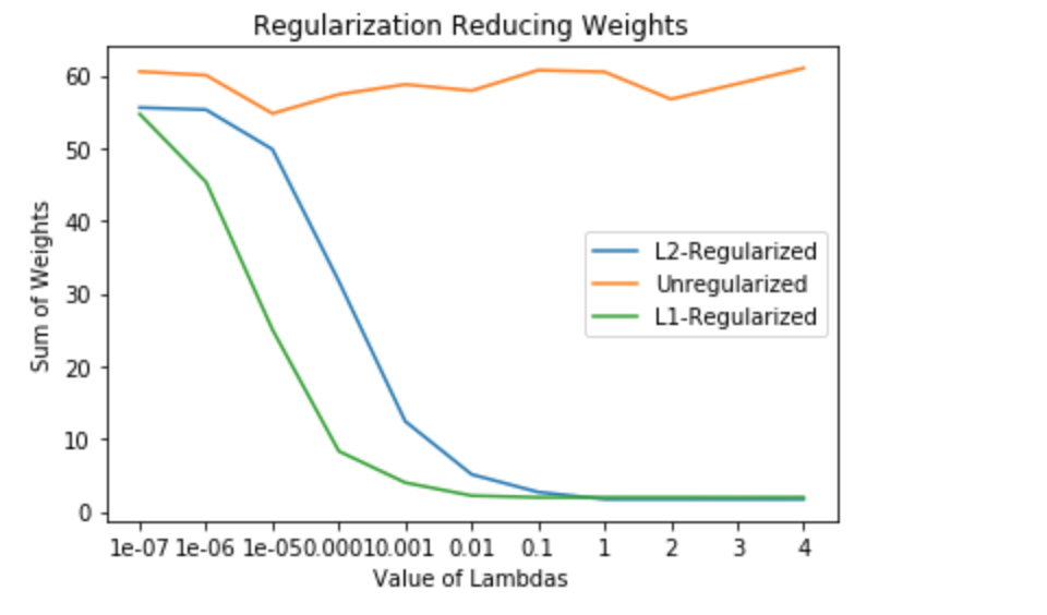 Weight decay in network weights based on lamda values
As we can see the lambda is the penalty and the weight is decayed as the value of penalty is increased.
Similarly out of 1 million parameters, I randomly sampled 5 weights and plotted their decay diagram with the value of regularization parameter. The results were what we expected:
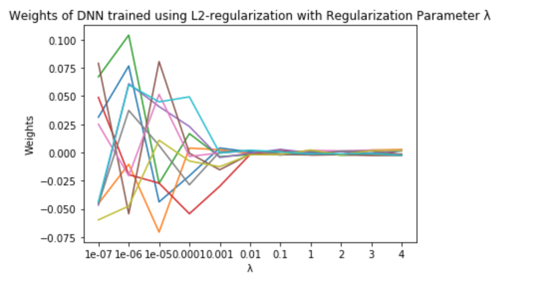 Weight decay in network weights with L2 regularization
 Weight decay in network weights with L1 regularization
And how a unregularized neural network looks like you asked?
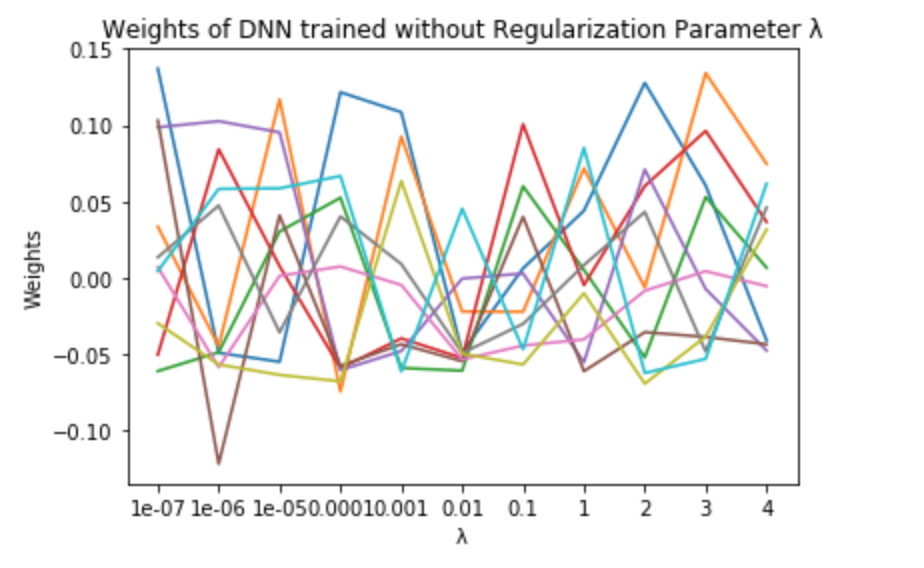 Weights of a DNN with no regularization
Feel Like spider man after these . Well that is for this post. Hope it was fun for you too as much as it was fun for me :D