
(Migrated from old blog)
I started with Deep Learning when PyTorch was already a big name and with extensive community support, which is just growing every day the more I use it the more I fall in love with it as a whole package to do my thing and the best part is, even if there is no functionality already available for my specific use case I can always write something myself because all of PyTorch code is nothing but just pure python.
There is a lot of hype with TensorFlow 2.0 too but as much as I have seen/used it, I still use Tensorflow just because of my familiarity with it as when I started it was still TensorFlow 1 time where there were static computation graphs which made it much difficult for beginners to start with and debug an already hard to debug somewhat black box system of Deep Learning. Also, why I love PyTorch is because it is simply more Pythonic! I will be talking a lot about PyTorch these days!!
Now it is amazing how similar the coding style of both the frameworks are and it is helping an end-user (the developer in this case) not to waste too much time choosing rather jumping onto the implementation.
What are Computation Graphs?
Alright, let’s also have some short introduction about something that I said earlier; so computation graphs what a fancy word but what is it means? Computation Graphs is basically how your deep learning model is represented in the system to put it formally.
A computational graph is a type of directed graph where nodes describe operations, while edges represent the data (tensor) flowing between those operations
As shown in the figure below
It helps you to represent the functional description of the, it is very handy when it comes to forward pass of the model, and even during backward pass it makes it very handy to pass the gradients.
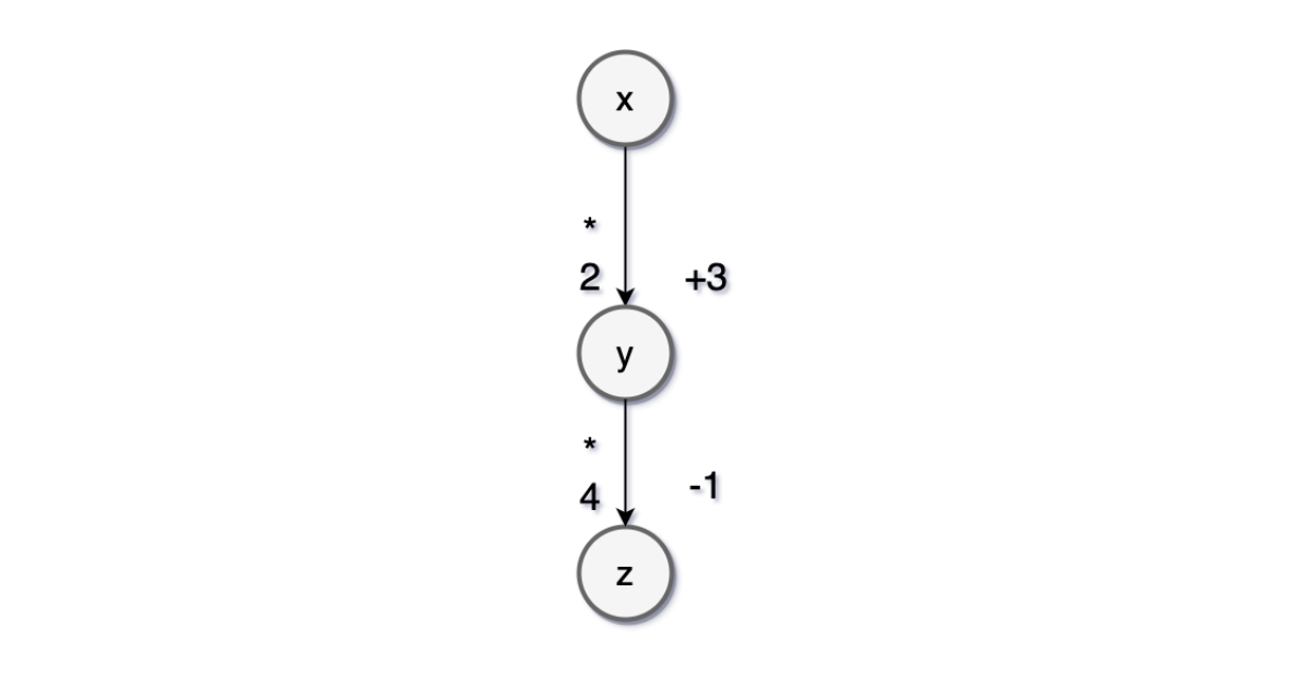 An Illustration of Computation Graph
Let’s look at some of the fun things first let’s talk about something called a node.
Let’s look at some basic definitions first:
- A node is a {tensor, matrix, vector, scalar} value where that is at the beginning of the graph.
- A leaf node means that no operation tracked by the gradient engine created it. Generally, in neural networks, these are the weights or inputs.
- An edge represents a function argument (and also data dependency).
- A node with an incoming edge is a function of that edge’s tail node.
- A node knows how to compute its value and the value of its derivative w.r.t each argument (edge) times a derivative of an arbitrary input
They are just pointers to nodes, a PyTorch implementation of the above computation graph will be
1
2
3
4
5
6
7
8
9
10
11
12
13
14
15
16
17
18
19
20
21
>>> import torch
>>> x = torch.randn([3,3], requires_grad=True)
# tensor([[-0.3360, -0.2482, -1.1120],
#         [ 1.7921,  0.1434, -0.8937],
#         [-1.0977,  1.2902,  1.3045]], requires_grad=True)
>>> y = 2 * x + 3
>>> y
# tensor([[2.3281, 2.5035, 0.7760],
#         [6.5842, 3.2868, 1.2125],
#         [0.8045, 5.5803, 5.6090]], grad_fn=<AddBackward0>)
>>> y = torch.randn([3,3], requires_grad=True)
>>> y
# tensor([[ 0.1635,  1.0521, -0.3305],
#         [-0.1648, -0.3370, -0.1706],
#         [-0.6183,  1.1766,  0.4418]], requires_grad=True)
>>> z = 4 * y - 1
>>> z
# tensor([[ 8.3123,  9.0141,  2.1038],
#         [25.3369, 12.1474,  3.8501],
#         [ 2.2181, 21.3214, 21.4362]], grad_fn=<SubBackward0>)
>>> z.sum().backward()
Notice the grad_fn this is where the whole graph is attached to the Tensor and all you have to differentiate or go backward is .backward() at a scalar and we have it. Simple and powerful! Right!
It will automatically go back and with the help of probability chain rule calculate the gradients in a reverse manner
\[\dfrac{\partial z}{\partial x} = \dfrac{ \partial z}{\partial y } \ast \dfrac{\partial y}{\partial x} = \dfrac{\partial(4y - 1)}{\partial y} = \dfrac{\partial (2x + 3)}{\partial x} = 4 \ast 2 = 8\]and if we check gradients of x by typing x.grad we get
1
2
3
4
>>> x.grad
# tensor([[8., 8., 8.],
#         [8., 8., 8.],
#         [8., 8., 8.]])
Perfect! Did you see how easy it makes things do
Let’s again go through how the algorithm works
- Creates computation graphs: Generates a computation graph or creates one on the fly
- Forward Loop: It loops over the nodes in topological order and keeps on computing its value based on the input and based on the input it generates a prediction (which can be later used to find loss w.r.t to their target values)
- Backward Propagation: It loops over the nodes in a reverse topological order starting with a final goal node, as discussed above it computes the derivatives of this final goal node wrt each leaf node. i.e how does my output change if I make a small change to the inputs.
Two Types of Computation Graphs
Static Computation Graphs: In this paradigm the graph is first constructed based on the defined architecture and then the mode is trained by running a bunch of data through this predefined graph. They are computationally faster but they are not very flexible when it comes to debugging.
Dynamic Computation Graphs: The graph is generated on the fly, PyTorch uses it. This allows us to change the architecture during runtime as the graph is created when the piece of code is run i,e the forward loop is run. They are relatively slower but are very useful while debugging as it is easier to locate the source.
So, I think this covers some basics of Computation Graphs and Automatic differentiation in PyTorch. Also, one thing worth noticing is that we can maybe in some cases want to turn off our Automatic differentiation or not bind the operation with our computation graph. In that case, we will use torch.no_grad() context and everything that will be within this context will not be added to the computation graph.
1
2
with torch.no_grad():
    # Your Custom code to implement
You can also put it as a decorator over a function to make them impact the autograd engine and deactivate it. It will reduce memory usage and speed up computations but you won’t be able to backprop.
1
2
3
@torch.no_grad()
def test_function(x):
   # do something with x
Let’s talk more about PyTorch and coding with it in further chapters of this PyTorch series. Till then have fun coding :)
Some nice reading materials/references to read more about it: