
(Migrated from old blog)
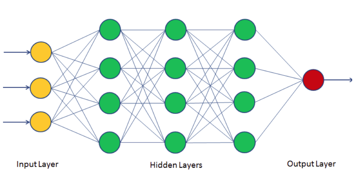
For those who read my logistic regression article, a neural network is somewhat kind of a similar thing with multiple layer architecture, even if you did not read not a big deal I will start from scratch. So consider this image, this is the best representation I found on the internet.
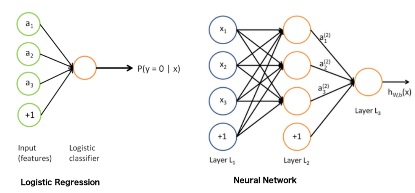 Logistic regression vs neural network
Difference between a logistic regression and Neural network in a Deep learning methodology
So the base of all neural network is an individual unit called neuron which is inspired from the neuron in the brain, we cannot yet model the complex recurrent nature in the actual bilogical neuron but this is our closest mathematical approximation and looks like (see fig. below)
Neuron in neural networks
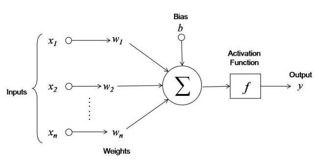 Artificial Neuron
Similar to the logistic regression and input to the neuron is the values x and it manages its own weights and bias and with its help, it outputs y after an activation function is applied to it. Mathematically,
\[a = \hat{y} = \sigma(z) = \sigma(WX + b)\]where $w$ is the weights to the input and b is the bias term to whether to activate a particular neuron or not. and X is the vector of input arrays $ X = [ x_1, x_2, x+3, … x_n ] $
These neurons are then stacked in layer and for each layer, we will use a superscript number in square braces to show what layer is being talked about $ z^{[1]} $
So mathematically a neural network looks like this,
\[z^{[1]} = W^{[1]}X + b^{[1]} \rightarrow a^{[1]} = \sigma{z^{[1]}} \rightarrow z^{[2]} = W^{[2]} a^{[1]} + b^{[2]} \rightarrow a^{[2]} = \sigma{z^{[2]}} \rightarrow L(a^{[2]} , y)\]where $L(a^{[2]} , y) $ is the loss function for a 2 layered architecture that has to be minimised.
So breaking these four equations down are all we need for a two-layered neural network architecture to work. First take the input array and pass it through the first layer by
\[z^{[1]} = W^{[1]}X + b^{[1]}\]then add the activation function of this layer i.e
\[a^{[1]} = \sigma{z^{[1]}}\]then the output of this layer i.e $ a^{[1]} $ will serve as the input to the next layer so the next layer becomes
\[z^{[2]} = W^{[2]} a^{[1]} + b^{[2]}\]and then we add the activation function to this in this scenario it is an sigmoid function, it can be any other activation function.
\[a^{[2]} = \sigma{z^{[2]}}\]Okay, Some Good math, for now, lets talk about some activation functions.
Activation Functions
Sigmoid Function
The activation function that we used for now was the sigmoid function it looks like, $$ \sigma(x) = \frac{1}{1 + e^{-x}} $
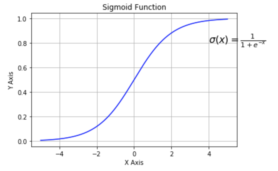 Sigmoid function
Extra: You can generate the same graph using python and matplotlib using this piece of code
1
2
3
4
5
6
7
8
9
10
11
12
import numpy as np
import matplotlib.pyplot as plt
def sigma(x):
    return 1 / (1 + np.exp(-x))
X = np.linspace(-5, 5, 1000)
plt.plot(X, sigma(X),'b')
plt.xlabel('X Axis')
plt.ylabel('Y Axis')
plt.title('Sigmoid Function')
plt.grid()
plt.text(4, 0.8, r'$\sigma(x)=\frac{1}{1+e^{-x}}$', fontsize=16)
plt.show()
Sigmoid is not used nowadays, it suffers the vanishing gradient problem, it is only used in the last layer of a binomial classification since the output it either 0 or 1.
Its derivation (useful in gradient descent) is
\[\sigma'(x) = \sigma(x)\left(1- \sigma(x)\right)\]TanH aka Hyperbolic Tangent
It is also a type of sigmoid function but generally has better performance than the default logit function mentioned above it ranges from $ [-1 , 1] $ unlike sigmoid that ranges from $ [0,1] $. $$ \tanh{(x)} = \frac{e^x - e^{-x}}{e^x + e^{-x}} $
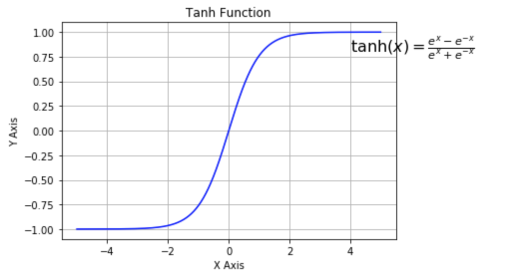 tanh activation function
tanh activation function
1
2
3
4
5
6
7
8
9
10
11
12
13
14
15
# Generate the graph of tanh function
import numpy as np
import matplotlib.pyplot as plt
%matplotlib inline

def tanh(x):
    return ( np.exp(x) - np.exp(-x)) / (np.exp(x) + np.exp(-x))

plt.plot(X, tanh(X),'b')
plt.xlabel('X Axis')
plt.ylabel('Y Axis')
plt.title('Tanh Function')
plt.grid()
plt.text(4, 0.8, r'$\tanh(x)=\frac{e^x - e^{-x}}{e^{x} +e^{-x}}$', fontsize=16)
plt.show()
Tanh is a better reference than the sigmoid (logit) function except for the case of the output layer of binary classifiers. It also suffers from the vanishing gradient problem.
Its derivation (useful in gradient descent) is
\[\tanh'(x) = 1 - \left( tanh(x) \right)^2\]Relu or Rectified Linear Activation Function
Relu is the most popular choice from the activation function now since it is least effective from the vanishing gradient problem. $$ \mathbb{Relu}(x) = \max(0,x) $
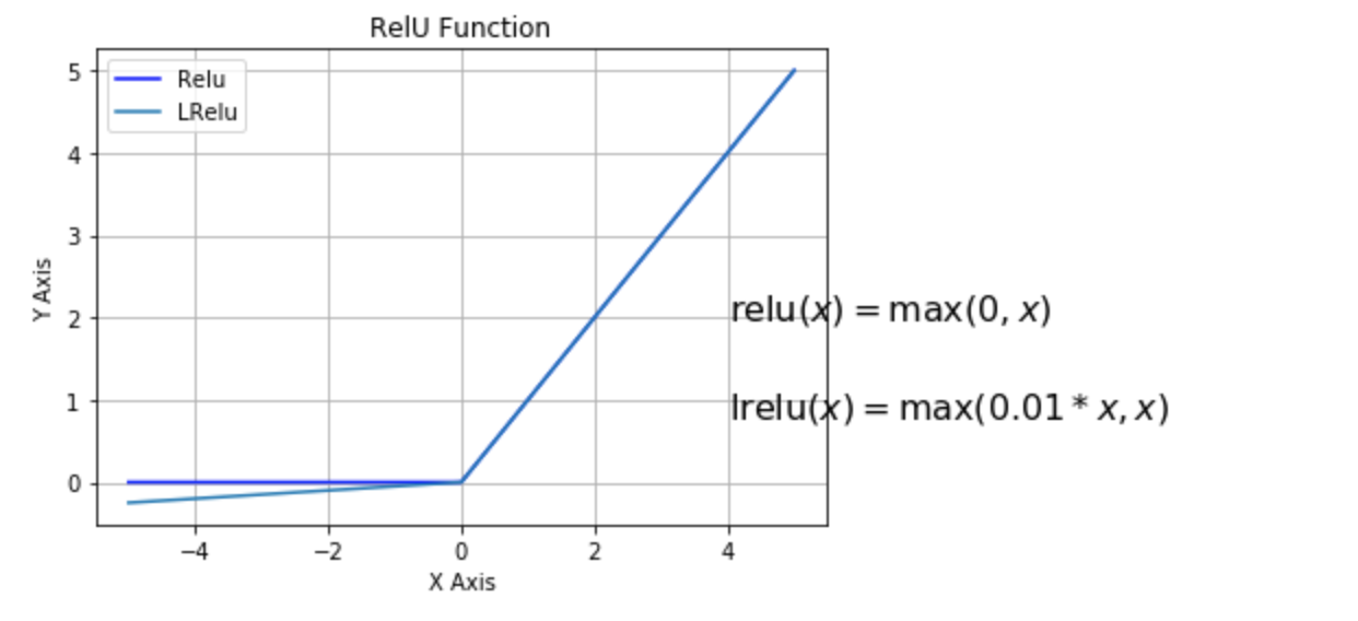 Relu and leaky relu activation functions
There is one variation of Relu called as leaky Relu which is almost similar but do sometimes provide little better results, even though people still tend to use relu more because it produces more the less same results. $$ \mathbb{LRelu}(x) = \max(0.1*x, x) $
1
2
3
4
5
6
7
8
9
10
11
12
13
14
15
16
17
18
19
20
21
import numpy as np
import matplotlib.pyplot as plt
%matplotlib inline

def relu(x):
    return np.maximum(x,0)

def lrelu(x):
    return np.maximum(0.01*x, x)

X = np.linspace(-5, 5, 1000)
plt.plot(X, relu(X),'b', label='Relu')
plt.plot(X, lrelu(X),'-', label='LRelu')
plt.xlabel('X Axis')
plt.ylabel('Y Axis')
plt.title('RelU Function')
plt.grid()
plt.legend()
plt.text(4, 0.8, r'$\operatorname{lrelu}(x)=\max(0.01*x,x)$', fontsize=16)
plt.text(4, 2, r'$\operatorname{relu}(x)=\max(0,x)$', fontsize=16)
plt.show()
Its derivation (useful in gradient descent) is
\[\mathbb{Relu}(x) = \begin{cases} 0 & {if }\ x<0 \\ 1 & {if }\ x \geq 0 \end{cases}\]and for leaky Relu it becomes
\[\mathbb{LRelu}(x) = \begin{cases} 0.01 & {if }\ x<0 \\ 1 & {if }\ x \geq 0 \end{cases}\]